return to the main page "Calculus I for Management"
return to the section "Exponential Functions & Marginal Analysis"
Worked-Out Exercises: Exponential & Logarithmic Functions - Part II
The following set of exercises is given together with hints, solutions, and solution paths. They are designed such that
you can first try to solve them and in case you need help, please, open the "hints" section. For checking your
answer, please, open the "solution" section and for getting more details or checking your way of solving the
exercise, please, open the "solution path" section.
|
|
|
Exercise 1: Differentiation Practice |
| |
|
Differentiate the following functions
\[
{\bf{a)}} \quad f(x) \, = \, x \cdot \ln(x) - x \, , \qquad {\bf{b)}} \quad f(x) \, = \, \sin(\ln(x)) \, ,
\]
as well as
\[
{\bf{c)}} \quad f(x) \, = \, \log_{10}(1 + \cos(x)) \, , \qquad \text{and} \qquad
{\bf{d)}} \quad f(x) \, = \, \frac{{\rm{e}}^{-x} \cos^2(x)}{x^2 + x + 1}
\]
|
|
 Hint Hint
(please, click on the "+" sign to read more)
You will need product rule, chain rule and logarithmic differentiation.
|
|
Solution
(please, click on the "+" sign to read more)
a) ln(x)
b) \(\frac{\cos(\ln(x))}{x}\)
c) \(\frac{-\sin(x)}{\ln(10) \cdot (1 + \cos(x))}\)
d) - \(\left( \frac{x^2 + 3x + 1}{x^2 + x + 1} + 2 \tan(x) \right) \cdot \frac{{\rm{e}}^{-x} \cos^2(x)}{x^2 + x + 1}\)
|
|
Solution Path
(please, click on the "+" sign to read more)
a) With the aid of the product rule, we have
\begin{eqnarray*}
f'(x) & = & \ln(x) + x \cdot \frac{1}{x} - 1 \, \, = \, \, \ln(x) + 1 - 1 \, \, = \, \, \ln(x) \, .
\end{eqnarray*}
b) With the aid of the chain rule, we have
\begin{eqnarray*}
f'(x) & = & \cos(\ln(x)) \cdot \frac{1}{x} \, \, = \, \, \frac{\cos(\ln(x))}{x} \, .
\end{eqnarray*}
c) With \(\frac{\textrm{d}}{\textrm{d} \, x} \, \log_b(x) = \frac{1}{x \cdot \ln(b)}\) and the aid of the chain rule, we have
\begin{eqnarray*}
f'(x) & = & \frac{-\sin(x)}{\ln(10) \cdot (1 + \cos(x)} \, .
\end{eqnarray*}
d) With the aid of logarithmic differentiation, we first take logarithms of both sides of the equation and use the laws of logarithms to simplify:
\[
\ln(f(x)) \, \, = \, \, -x + 2 \ln(\cos(x)) - \ln(x^2+x+1) \, .
\]
Differentiating implicitly with respect to \(x\) gives
\[
\frac{1}{f(x)} \cdot f'(x) \, \, = \, \, -1 - 2 \frac{\sin(x)}{\cos(x)} - \frac{2x + 1}{x^2 + x + 1} \, \, = \, \,
-\frac{x^2 + 3x + 1}{x^2 + x + 1} - 2 \tan(x) \, .
\]
Next,
\[
\frac{1}{f(x)} \cdot f'(x) \, \, = \, \, -\frac{x^2 + 3x + 1}{x^2 + x + 1} - 2 \tan(x)
\]
gives the seeked derivative
\[
f'(x) \, \, = \, \, - \left( \frac{x^2 + 3x + 1}{x^2 + x + 1} + 2 \tan(x) \right) \cdot \frac{{\rm{e}}^{-x} \cos^2(x)}{x^2 + x + 1} \, .
\]
|
|
Exercise 2: Population Growth |
| |
|
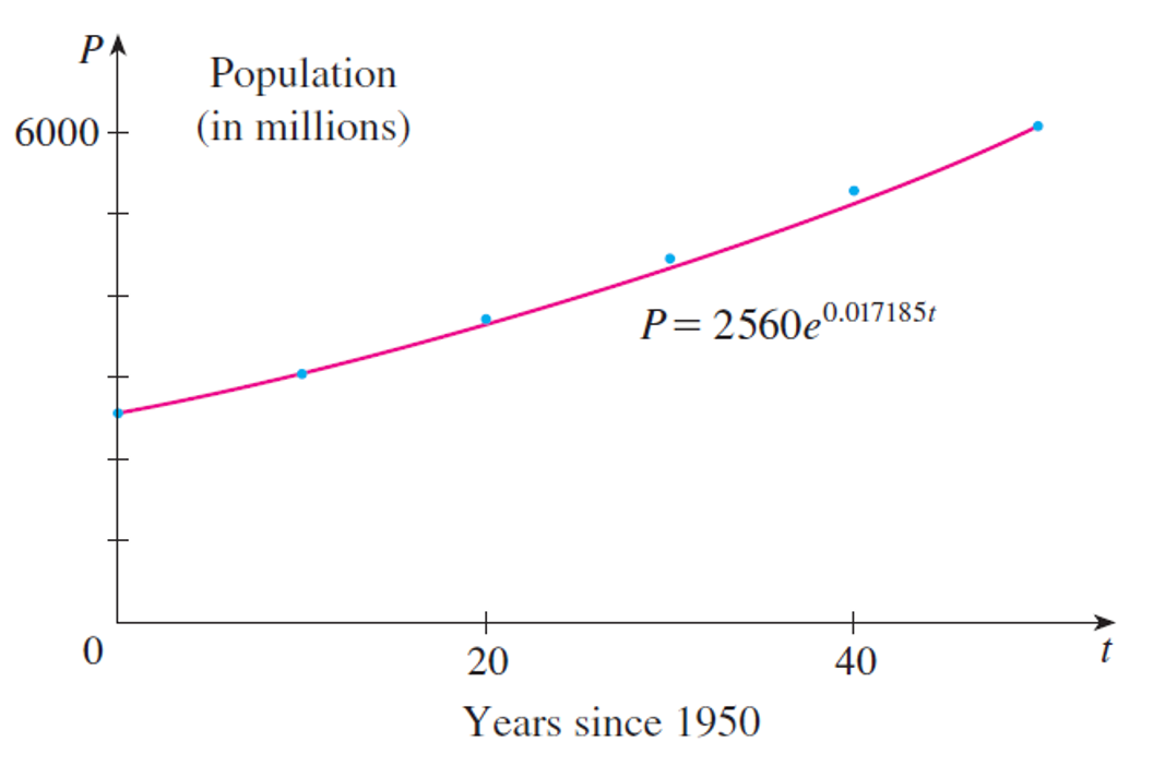
Use the fact that the world population was 2560 million in 1950 and
3040 million in 1960 to model the population of the world in the second half of the 20th
century. (Assume that the growth rate is proportional to the population size.)
What is
the relative growth rate? Use the model to estimate the world population in 1993 and to
predict the population in the year 2020.
|
|
Hint
(please, click on the "+" sign to read more)
assume that \(\frac{\textrm{d} \, P}{\textrm{d} \, t} = kP\)
|
|
Solution
(please, click on the "+" sign to read more)
The relative growth rate is about \(1.7\%\) per year.
The world population in 1993 was \(5360 \cdot 10^6 \) and in 2020, it will be \(8524 \cdot 10^6 \) .
|
|
Solution Path
(please, click on the "+" sign to read more)
We measure the time \(t\) in years and let \(t = 0\) in the year 1950. We measure
the population \(P(t)\) in millions of people. Then \(P(0) = 2560\) and \(P(10) = 3040\). Since
we are assuming that \(\frac{\textrm{d} \, P}{\textrm{d} \, t} = kP\), we have
\begin{eqnarray*}
P(t) & = & P(0) \, {\rm{e}}^{k t} \, \, = \, \, 2560 \, {\rm{e}}^{kt}
P(10) & = & 2560 \, {\rm{e}}^{10 k} \, \, = \, \, 3040
k & = & \tfrac{1}{10} \, \ln\left( \frac{3040}{2560} \right) \, \, \approx \, \, 0.017185 \, .
\end{eqnarray*}
The relative growth rate is about \(1.7\%\) per year and the model is
\[
P(t) \, \, = \, \, 2560 {\rm{e}}^{0.017185 t} \, .
\]
We estimate that the world population in 1993 was
\[
P(43) \, \, = \, \, 2560 {\rm{e}}^{0.017185 \cdot 43} \, \, = \, \, 5360 \cdot 10^6 \, .
\]
The model predicts that the population in 2020 will be
\[
P(70) \, \, = \, \, 2560 {\rm{e}}^{0.017185 \cdot 70} \, \, = \, \, 8524 \cdot 10^6 \, .
\]
The graph in the figure shows that the model is fairly accurate to the end of the 20th century
(the dots represent the actual population), so the estimate for 1993 is quite reliable.
But the prediction for 2020 is riskier.
|
|
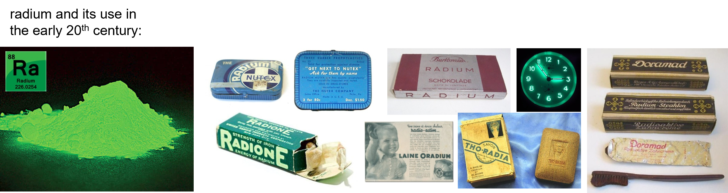
Exercise 3: Radioactive Decay |
| |
|
The half-life of radium-226 is 1590 years.
a) A sample of radium-226 has a mass of \(100\) \(mg\). Find a formula for the mass of the
sample that remains after \(t\) years.
b) Find the mass after \(1000\) years correct to the nearest milligram.
c) When will the mass be reduced to \(30\) \(mg\)?
|
|
Hint
(please, click on the "+" sign to read more)
Let \(m(t)\) be the mass of radium-226 (in milligrams) that remains after \(t\) years, then \(\frac{\textrm{d} \, m}{\textrm{d} \, t} = km\).
|
|
Solution
(please, click on the "+" sign to read more)
a) m(t)=\(100 \cdot 2^{-t/1590}\)
b) m(1000) =\( 100 \, {\rm{e}}^{-(\ln(2)) 1000/ 1590} \, \, \approx \, \, 65 \, \, \) [mg]
c) t = \(-1590 \frac{\ln(0.3)}{\ln(2)} \, \, \approx \, \, 2762 \, \, \) [years]
|
|
Solution Path
(please, click on the "+" sign to read more)
a) Let \(m(t)\) be the mass of radium-226 (in milligrams) that remains after \(t\) years. Then \(\frac{\textrm{d} \, m}{\textrm{d} \, t} = km\) and \(m(0) = 100\), so
\[
m(t) \, \, = \, \, m(0) \, {\rm{e}}^{kt} \, \, = \, \, 100 \, {\rm{e}}^{kt} \, .
\]
In order to determine the value of \(k\), we use the fact that \(m(1590) = \tfrac{1}{2} \cdot 100\). Thus
\[
100 \, {\rm{e}}^{1590 k} \, \, = \, \, 50 \qquad \text{so} \qquad {\rm{e}}^{1590 k} \, \, = \, \, \tfrac{1}{2}
\]
and
\[
1590 \, k \, \, = \, \, \ln(\tfrac{1}{2}) \, \, = \, \, -\ln(2) \qquad \Longrightarrow \qquad
k \, \, = \, \, -\frac{\ln(2)}{1590} \, .
\]
Therefore
\[
m(t) \, \, = \, \, 100 \, {\rm{e}}^{-(\ln(2))t/1590} \, .
\]
We could use the fact that \({\rm{e}}^{\ln(2)} = 2\) to write the expression for \(m(t)\) in the alternative
form
\[
m(t) \, \, = \, \, 100 \cdot 2^{-t/1590} \, .
\]
b) The mass after \(1000\) years is
\[
m(1000) \, \, = \, \, 100 \, {\rm{e}}^{-(\ln(2)) 1000/ 1590} \, \, \approx \, \, 65 \, \, \, [mg] \, .
\]
c) We want to find the value of \(t\) such that \(m(t) = 30\), that is,
\[
100 \, {\rm{e}}^{-(\ln(2)) t/ 1590} \, \, = \, \, 30 \qquad \text{or} \qquad {\rm{e}}^{-(\ln(2)) t/ 1590} \, \, = \, \, 0.3 \, .
\]
We solve this equation for \(t\) by taking the natural logarithm of both sides:
\[
-\frac{\ln(2)}{1590} \, t \, \, = \, \, \ln(0.3) \qquad \Longrightarrow \qquad t \, \, = \, \, -1590 \frac{\ln(0.3)}{\ln(2)} \, \, \approx \, \, 2762 \, \, \, [\text{years}] \, .
\]
|
|
|
Copyright Kutaisi International University — All Rights Reserved — Last Modified: 12/ 10/ 2022
|
|
| |