Mathematics for Management -- Supplementary Electronic Materials

return to the main page "Calculus I for Management"
return to the page "Applications of Integration"

Worked-Out Exercises: Applications of Integration in Economics

The following set of exercises is given together with hints, solutions, and solution paths. They are designed such that you can first try to solve them and in case you need help, please, open the "hints" section. For checking your answer, please, open the "solution" section and for getting more details or checking your way of solving the exercise, please, open the "solution path" section.


Exercise 1: Gini indices for given Lorenz curves

Find the Gini index for the given Lorenz curve: \[ L_1(x) \, \, = \, \, x^3 \qquad \text{and} \qquad L_2(x) \, \, = \, \, \tfrac{2}{3} x^{3.7} + \tfrac{1}{3} x \, . \]

Hint (please, click on the "+" sign to read more) Recall, that Gini Index is given by the formula \[ GI \, \, = \, \, 2 \int^1_0 \left( x - L(x) \right) \textrm{d} x \, . \]

Solution (please, click on the "+" sign to read more) $G_1 = \, \, \tfrac{1}{2}\\ $ $G_2 = \, \, 0.1914894 $

Solution Path (please, click on the "+" sign to read more) The respective Gini indices are $ \begin{eqnarray} G_1 & = & 2 \int^1_0 \left( x - x^3 \right) \, \, = \, \, 2 \Big[ \tfrac{1}{2} x^2 - \tfrac{1}{4} x^4 \Big]^1_0 \, \, = \, \, \tfrac{1}{2}\\ G_2 & = & 2 \int^1_0 \left( x - (\tfrac{2}{3} x^{3.7} + \tfrac{1}{3} x) \right) \, \, = \, \, 2 [ \tfrac{1}{3} x^2 - \tfrac{2}{3 \cdot 4.7} x^{3.7} \Big]^1_0 \, \, = \, \, 0.1914894 \end{eqnarray}$

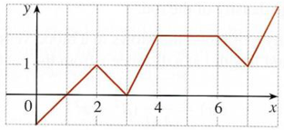
Exercise 2: The average of a function

Find the average value of $f$ on $[0,8]$.

Hint (please, click on the "+" sign to read more) We compute the average, by summing up discrete weighted averages and then divide by $8$

Solution (please, click on the "+" sign to read more) $1$

Solution Path (please, click on the "+" sign to read more) We compute the average, by summing up discrete weighted averages and then divide by $8$: $\begin{eqnarray} f_{\textrm{avg}} & = & \frac{0 \cdot 2 + \tfrac{1}{2} \cdot 1 + 1 \cdot 1 + 2 \cdot 2 + \tfrac{3}{2} \cdot 1 + 1 \cdot 1}{8} \\[2mm] & = & \frac{8}{8} \, \, = \, \, 1 \end{eqnarray}$

Exercise 3: Finding the average value

Graph the function \[ f(x) \, \, = \, \, x^2 \, - \, 1 \qquad \text{on $[0, \sqrt{3}]$} \, , \] and find its average value over the given interval.

Hint (please, click on the "+" sign to read more) Recall, that \[ f_{\text{avg}} \, \, = \, \, \frac{1}{b-a} \int^b_a f(x) \, \textrm{d} x \, . \]

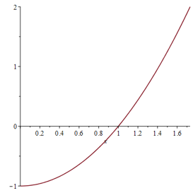
Solution (please, click on the "+" sign to read more) $f_{\textrm{avg}} = 0$

Solution Path (please, click on the "+" sign to read more) We have $\begin{eqnarray} \frac{1}{\sqrt{3}} \, \int^{\sqrt{3}}_0 \left( x^2 - 1 \right) \textrm{d} x & = & \frac{1}{\sqrt{3}} \, \Big[ \tfrac{1}{3} x^3 - x \Big]^{\sqrt{3}}_0 \\[2mm] & = & \frac{1}{\sqrt{3}} \left( \left( \tfrac{1}{3} \cdot 3 \cdot \sqrt{3} - \sqrt{3} \right) - 0 \right) \\[2mm] & = & 0 \end{eqnarray}$

Exercise 4: Future and present value of an annuity

An annuity pays a continuous income stream of $M$ GEL per year into an account that pays interest at an annual rate $r$ compounded continuously for a term of $T$ years. ${\bf{a)}}$ Show that the future value $FV$ of the annuity is \[ FV \, \, = \, \, \tfrac{M}{r} \left( {\rm{e}}^{rT} - 1 \right) \, . \] ${\bf{b)}}$ Show that the present value $PV$ of the annuity is \[ PV \, \, = \, \, \tfrac{M}{r} \left( 1 - {\rm{e}}^{-rT} \right) \, . \]

Hint (please, click on the "+" sign to read more) Recall, that future value $FV$ of the income stream over the term $T$ is given by the definite integral \[ FV \, \, = \, \, \int^T_0 f(t) {\rm{e}}^{r(T-t)} \, \textrm{d} t \, \, = \, \, {\rm{e}}^{rT} \int^T_0 f(t) {\rm{e}}^{-rt} \, \textrm{d} t \] and the present value $PV$ of an income stream that is deposited continuously at the rate $f(t)$ into an account that earns interest at an annual rate $r$ compounded continuously for a term of $T$ years is given by \[ PV \, \, = \, \, \int^T_0 f(t) {\rm{e}}^{-rt} \, \textrm{d} t \, . \]

Solution (please, click on the "+" sign to read more) This exercise does not come with the correct answer since it only requires to show that given formula is correct.

Solution Path (please, click on the "+" sign to read more) ${\bf{a)}}$ The future value $FV$ of the anuity is $\begin{eqnarray} FV & = & \int^T_0 \, M {\rm{e}}^{r(T-t)} \, \textrm{d} t \, \, = \, \, M {\rm{e}}^{rT} \int^T_0 \, {\rm{e}}^{-rt} \, \textrm{d} t \, \, = \, \, M {\rm{e}}^{rT} \Big[ -\tfrac{1}{r} {\rm{e}}^{-rt} \Big]^T_0 \\[1mm] & = & M {\rm{e}}^{rT} \left( -\tfrac{1}{r} {\rm{e}}^{-rT} + \tfrac{1}{r} \right) \, \, = \, \, \tfrac{M}{r} \left( {\rm{e}}^{rT} - 1 \right) \end{eqnarray}$ ${\bf{b)}}$ The present value $PV$ of the anuity is $\begin{eqnarray} PV & = & \int^T_0 \, M {\rm{e}}^{-rt} \, \textrm{d} t \, \, = \, \, \dots \, \, = \, \, M \left( -\tfrac{1}{r} {\rm{e}}^{-rT} + \tfrac{1}{r} \right) \\[1mm] & = & \tfrac{M}{r} \left( 1 - {\rm{e}}^{-rT} \right) \end{eqnarray}$

Exercise 5: Consumers' willingness to spend

For the consumers' demand functions $D(q) = 2 (64 - q^2)$ GEL per unit find the total amount of money consumers are willing to spend to obtain $q_0 = 6$ units of the commodity.

Hint (please, click on the "+" sign to read more) Recall, that the total consumer willingness $WS$ is \[ WS \, \, = \, \, \int^{q_0}_0 D(q) \, \textrm{d} q \, \, \]

Solution (please, click on the "+" sign to read more) $624$ GEL

Solution Path (please, click on the "+" sign to read more) The total consumer willingness $WS$ to spend for $q_0 = 6$ units is \[ WS \, \, = \, \, \int^{q_0}_0 D(q) \, \textrm{d} q \, \, = \, \, \int^6_0 \, 2 (64 - q^2) \, \textrm{d} q \, \, = \, \, \Big[ 128 q - \tfrac{2}{3} q^3 \Big]^6_0 \, \, = \, \, 624 \, . \] So consumers are willing to pay $624$ GEL for as many as $6$ units.

Exercise 6: Consumers' surplus

Let $p = D(q) = 2(64-q^2)$ be the price (GEL per unit) at which $q$ units of a particular commodity will be demanded by the market (that is, all $q$ units will be sold at this price). Find the price $p_0 = D(q_0)$ at which $q_0 = 6$ units will be demanded and compute the corresponding consumers' surplus $CS$.

Hint (please, click on the "+" sign to read more) Recall, that the consumers' surplus $CS$ is \[ CS = \int^{q_0}_0 D(q) \, \textrm{d} q - p_0 q_0 \, \,\]

Solution (please, click on the "+" sign to read more) $288$ GEL.

Solution Path (please, click on the "+" sign to read more) For $q_0 = 6$ we have $p_0 = D(6) = 56$. Thus, the seeked consumers' surplus $CS$ is \begin{eqnarray} CS & = & \int^{q_0}_0 D(q) \, \textrm{d} q - p_0 q_0 \, \, = \, \, \int^6_0 \, 2 (64 - q^2) \, \textrm{d} q - 6 \cdot 56 \\[1mm] & = & \Big[ 128 q - \tfrac{2}{3} q^3 \Big]^6_0 - 336 \, \, = \, \, 288 \, . \end{eqnarray} So the consumers' surplus is $288$ GEL.